This is my blog. I’ll be writing about topics which interest me: stuff related to biology, medicine, life sciences, etc. I hope you will enjoy reading my posts and subscribe below to get notified when I post new updates.
Second year of medicine at KCL brings many new experiences and opportunities- going to hospital wards, doing more clinical skills, conducting research and joining committees of student societies. Student societies offer the chance to develop one’s soft skills and technical knowledge, not to mention meeting people with similar interests and connecting with experts in a particular field. Luckily, I was able to join a society that is all about a topic of medicine I love- surgical innovation!
Surgical Innovation is a fascinating field combining the inherent intricacy of surgery with the fast-paced and ever-changing world of technology. It also offers surgeons the opportunity to contribute to better patient outcomes in more than one way. Surgical Innovation is also a massively broad domain involving Virtual Reality, Machine Learning, Nanotechnology and Robotics (my favourite!).
But back to the society- like everyone else, we’ve got a president, vice president, secretary, treasurer and officers with roles managing events, social media, diversity and equality and sponsorships. I’m an events officer, a role I really enjoy since it gives me a very active role in society activities and allows me to contact and connect with experts in academia, clinic and industry.
Our first major activity as a society was putting up a stall at the KCL Welcome Fair on the 22nd of September. As a new society, it was really important for us to make our presence felt. We needed to have something really exciting so that students would come to our stall and express interest. That’s where the 3D printer came in- I was able to organise a demonstration after contacting the Biomedical engineering and imaging sciences department headed by Professor Kawal Rhode. He and his PhD students very graciously helped us arrange for it to be at our stall.
Our 3D printer with an array of small models in front of it
The 3D printer was able to print hearts, a cross section of a spinal vertebrae, brains, aortas, and KCL badges. We were able to attract many curious students from various STEM fields. It was a highlight for me too- I’ve been dabbling in the world of robotics and was very interested to see the printer’s delta platform at work.
Our stall at the welcome fair- I’m on the right next to our amazing president!
The software side of the printer was quite amazing- it would take the model we wanted it to print and superimpose it in 3D coordinate space. It would then represent every point of the model using three coordinates and convert these coordinates into language the printer software can understand. The process is very similar to how robot kinematics work when determining a joint’s position and orientation. I kept a brain as a little memento of the welcome fair-
My model of the human brain; I was about to caption it as ‘my little brain’ when I realised what that sounded like
After our initial success, we turned our minds towards our first event which happened on October 3rd. We were very fortunate to have two legendary figures in the world of surgical innovation come to talk at our event- Professor Prokar Dasgupta and Dr. Angela Lam. Prof. Dasgupta, who is foundation professor of surgery at King’s Health Partners and recent Padma Shri awardee, gave us a talk on the importance of innovation in medicine, introducing us to many new and upcoming technologies that have the potential to change common practices in surgery.
Dr. Angela Lam, Innovation lead for ASIT, co-founder of the National MedTech foundation and a core surgical trainee delivered a talk on ways through which one can get involved in surgical innovation at early stages in our medical education. Her talk was very practical, answering many of my questions regarding the realities of pursuing a more entrepreneurial/innovator route as a medic.
At the end of the event, Prof. Dasgupta took us to Guy’s Chapel, where he introduced us to the grave of Astley Cooper, an accomplished surgeon of the 19th century. He then told us about a rather interesting and highly inspirational person who had trained under Astley Cooper- Margret Ann Buckley, better known as James Barry. In order to pursue a career as a surgeon in a day when women were barred from studying medicine, Buckley turned herself into James Barry and went on to have an illustrious career in the British Army. Among her many accomplishments was the first ever recorded Caesarean Section by a European in Africa. Prof. Dasgupta reminded us that we were standing in the very place where innovators like James Barry stood, and asked us to take this as an inspiration and do are best to be effective innovators who would work to improve patient outcomes.
Professor Dasgupta delivering his talk
Dr. Lam’s talk on getting involved in innovation at an early stage in our careers
A picture of everyone at the event- The committee is at the front (I’m standing with a white shirt and a big smile!), flanked by Dr. Lam, Prof. Dasgupta and Dr. Ata Jaffer from left to right.
All in all, I’ve really enjoyed being part of the society till now. i’ve met some great people who share my interests in surgery, gained a lot more knowledge about the domain and have also got some fascinating opportunities through our events. Indeed, my next blog post will be on one such opportunity I got- shadowing the wonderful Dr. Ata Jaffer, a Urology registrar and robotic surgeon!
A little teaser of my next blog post- me in theatre with a Da Vinci Surgical robot!
Surgery and Scotland have a historic relationship- indeed, many famous surgeons such as Robert Liston, John Hunter and Charles Bell hail from the nation. While visiting Scotland, I found out about the Surgeons’ Hall museums at Royal College of Surgeons Edinburgh and couldn’t give it a miss!
Outside the museum
The museum has four components- a history of surgery section, the Wohl pathology museum, a large dental collection and the body voyager gallery.
The history of surgery section contained some interesting surgical tools dating back to the 18th and 19th-centuries. One often doesn’t realise how far we have progressed in surgery till one looks at surgical practices from two hundred years ago. At that time, surgeries were largely limited to amputations, performed without antiseptic or anesthetic. Surgeons would wear the same coat for every operation, every blood stain on it like a badge of honour. Mortality rates were high- one surgery performed in this period led to a 300% mortality rate when the surgeon, his assistant and the patient all died of infection!
A 19th-century surgery – no antiseptic, anesthetic or surgical gowns. The surgeons here are wearing coats similar to one displayed in the museum.
An 18th century surgeons most important instrument- a saw.
Interestingly, surgery started as a part-time profession for barbers. Skilled with razors, barbers would perform amputations and bloodletting for patients using crude saws and curved knives. It was only in the 18th-century that a distinction between the two became widespread. Surgeons were initially looked down upon by physicians, who believed that intentionally cutting into the body was contrary to the ethos of a medical practitioner.
A medieval barber-surgeon on his duties
I also learned about the gruesome Burke and Hare murders- as 19th-century anatomists began phasing out knowledge acquired through ancient textbooks and explored the body on their own, they encountered a problem- there was a lack of cadavers to dissect. Without any legal method to obtain fresh bodies for dissection, surgeons had to turn to ‘bodysnatchers’ who would remove fresh corpses from their graves to sell to surgeons. For Burke and Hare, however, snatching dead bodies wasn’t enough. Over ten months, they committed sixteen murders in Edinburgh and sold off the bodies to surgeon Robert Knox until they were caught.
The infamous Burke and Hare duo
This section also had a very informative anatomy theatre where a 19th-century surgeon walked visitors through the first legal dissection in Edinburgh. It also had some rare specimens, including a femur that had grown to the size of a melon after being untreated for an infection.
The Wohl Pathology Museum was divided into roughly ten surgical specialties, with a plethora of specimens displaying interesting medical conditions. I was really happy to be able to use some of my knowledge from my first year to recognise anatomical landmarks and better understand certain diseases. I was happy to see a familiar name in the museum- Hodgkin! Hodgkin’s lymphoma is a disease that (in its later stages) causes lesions in the Liver. KCL’s medical school building is also named Hodgkin (both the condition and the building are named after Thomas Hodgkin, an alumnus of King’s). I spent some time looking at aneurysms- after having seen a massive abdominal aortic aneurysm during dissections, the condition has become one of great interest to me. The lower floor of the pathology museum also had a section for military medicine that I thoroughly enjoyed seeing.
One aspect of the museum I really liked was that it included both the past and the future of surgery. The body voyager exhibit, which focused on modern surgery, had some fascinating displays of 21st-century minimally invasive surgical instruments, robotic systems, information on keyhole surgery procedures and simulations. One entertaining machine could measure your hand tremor to see if you would make a good neurosurgeon. Another involved guiding a virtual surgical tool into the brain using a joystick.
The museum’s highlight was a master robot from a demo Da-Vinci Surgical system that was installed to allow visitors to experience first-hand the work of a robotic surgeon. I imagine that it’s rare for a medical student to get the opportunity to try out a real robotic surgical system (albeit a demo one), so I was very, very glad to get this chance. What surprised me the most was how fluid the master robot manipulator was- the experience was akin to slicing through butter. Although the end effector placement was a bit challenging to understand, the robot could match every input I gave it. In time, I was able to develop a rough understanding of the arm movements and was successful in drawing a tree on the virtual paint-board being used to demonstrate the robot’s working. I also loved the Endowrist system display- I’m currently trying to learn the basics of robotics, so a demonstration of the mechanical basis of the manipulator was very interesting. A side note- the Endowrist system has more degrees of freedom than a human wrist, making it particularly dextrous!
An opened up EndoWrist like the one displayed in the museum. Credit to –link
All in all, I really loved my visit to RCSEd. I wasn’t able to take any pictures inside the museum, but the things I learned about the history of surgery and the fun experiences I had in the body voyager exhibit will stay with me and motivate me to achieve my dream of becoming a successful surgeon and innovator.
A bench in the college’s garden dedicated to the work of surgeons in the battlefield. Mary, Queen of Scots, was the first Scottish monarch to declare that during war, medical practitioners treating their respective armies would be considered non-combatants.
Modern surgery, with it’s ability to perform invasive procedures in a controlled manner to treat patients is a hallmark of human progress. Surgery involves so many professionals with different areas of expertise working together to ensure that a patient’s treatment goes smoothly. I myself have always been keen on learning more about it, but as a first year, it isn’t very easy to get surgical experience. However, it is events such as KCL Surgical Society’s annual 2022 conference which allow students like me to get a glimpse into what surgery is really about.
The conference had five workshops in total- two in the morning (a choice of two workshops out of basic suturing, CST portfolio and speed dating a surgeon) and three in the afternoon (plastics, vascular and orthopaedics). I chose CST portfolio and basic suturing since I was really interested in those two topics. There was never a dull moment during the day- the organisation, logistics and planning of the conference were flawless and gave us all an opportunity to work and interact with students from various stages of medical education.
The first workshop I attended was on creating a good portfolio for your Core Surgical Training (CST) applications. Of course, as a first year I am still far away from that stage in my career. However, I’ve always been curious about the qualities and skills that assessors look for and felt that this workshop would be perfect to understand that.
One important takeaway here was that it is crucial to keep a track of everything you do. Keep an account of the conferences you attended, roles you undertook, times when you assisted in surgery, etc. If you maintain a record of these activities (for instance, in form of a log book containing the surgeries you participated in) it helps accumulate those points without having to do everything in a rush when the application deadline comes close.
Another important takeaway was that you shouldn’t be afraid to seek out opportunities. Actively search for them and don’t hesitate when approaching people or organisations. Quickly grab opportunities to do research, present your project as an abstract or a poster or apply for prizes if you find any. The worst you can get in the form of a response is a ‘no’ and many times you’re one of the few who actually applied!
I really enjoyed the conference’s emphasis on practical skills. For a first year medicine student, the opportunity to learn suturing isn’t just a great way to build those skills- it’s also very inspirational. I’ll have to admit, it wasn’t very easy at first. In my right hand was a pair of locking forceps and in the other toothed forceps. It was a bit like being a warrior of the old, sword in one hand and shield in another. There was a constant battle between getting my needle in the correct angle and ensuring that my knots didn’t untie themselves. The frequent guidance provided by the instructors at the conference really helped build confidence with suturing, and soon I could tie knots without worrying about getting my forceps tied up with them.
The continuous sutures I made during the morning basic suturing workshop
Here’s me with my sutures!
Making Kessler knots while repairing pig foot tendons during the plastics workshop was probably the most difficult of them all- thanks to the clear diagrams used by the instructors to explain, the technique became much clearer.
The Orthopaedics workshop was really fun! We got to simulate the repairing of a femoral neck fracture using a variety of instruments. I feel that my appreciation for a surgeon’s work increased greatly during this workshop. I was struggling to maintain my drill’s position and regularly held on to the bone to get a better grip. Surgeons don’t have this option- they can only access the bone through a cut in the thigh. Instead, they have to orient themselves using X-rays and other imaging devices. Along with this, they’ve got to have good strength and stamina- those drills were really heavy!
The orthopaedic workshop setup
The Vascular workshop was another highly informative session. Apart from learning the technique behind patch angioplasties we also got the opportunity to learn how to tie surgical knots. It took a bit of time to understand, but eventually I got the hang of it. I’m planning to practice it regularly so that I don’t forget!
We used a rubber pipe as an artery and a piece of band-aid to simulate the patch
All in all, the conference was really informative and interesting to attend. Along with learning a number of technical skills, I was able to interact with surgeons from different specialities and understand a bit more about their work. I hope that I’ll get to experience amazing conferences like this again while at medical school and am looking forward to the next exciting event planned for us!
It’s been a long time since I’ve updated my blog- applying to and then joining university has been fun and interesting, but time has been rather limited. However, I’ve recently taken up learning a skill that I have found to be very exciting and worth writing about – coding.
Of course, coding isn’t something that immediately comes to mind when one looks at a blog related to life science. I myself believed (until about six months ago) that coding and an understanding of Machine Learning (ML) wasn’t required for someone going into medicine. However, I realised that that is a rather foolish approach to take- ML has already begun to revolutionise healthcare in ways we couldn’t have possibly imagined.
Thus, I decided to try to learn Python. This was about six months ago, and while I have learned a great deal, I know that there is a long way to go till I’ll be proficient in the language. This isn’t the first time I’ve tried to learn how to code – I did do a small project around two years ago (I wrote about that as well – link) but it was basic and I didn’t really get motivated enough to explore further. It’s different this time – I am really motivated!
And now to my project. I have made a program that will be able to predict pneumonia by looking at chest X-rays with reasonable accuracy. Since this was my first project, I did come across countless little problems that took time to solve. One particular issue I’ll be talking about later took me two weeks to resolve! But that’s the great thing really- not only did I learn and explore different areas of Python and PyTorch (the python library I used for predictions) but also learned how to handle errors.
This project is catered towards students studying medicine/healthcare related fields. The reason why I’ve used transfer learning is that you don’t need to actually create a model by writing countless lines of code- you can simply import and apply ResNet50 (a Deep Convolutional Neural Network (CNN)) in a very simple and efficient manner. I’ve also talked a bit more about how I feel ML might impact healthcare, so if that’s something you find particularly interesting feel free to scroll down to the penultimate section.
The first step – importing libraries, data preparation and augmentation
The first step is to import our libraries. You might have to download these using the command !pip install library_name if you aren’t working on Colab.
Another thing to look at is that I’m using the library PyTorch. PyTorch is one of three main libraries made for neural networks (the other two are Tensorflow and Keras). I’ve chosen PyTorch primarily because it is more explainable – it’s easier to understand how the code works and how the model makes its decisions (this is the main reason why PyTorch is more prevalent in academia/research). Keras and Tensorflow are, however, said to be more powerful than PyTorch.
Explainability is particularly important in medicine. We have these amazing, powerful algorithms and we know that they can give us some great results. However, we still aren’t sure about how these algorithms work, make decisions or make predictions. This lack of clarity has led to such algorithms being termed as ‘black-box’ algorithms, and has also resulted in a general feeling of distrust with regards to results obtained from these algorithms. Doctors may tend to disregard results obtained by ML because they cannot understand how it arrived at that result (indeed, no one really can!). You can improve explainability by making your code easier to understand, including graphs and using Python libraries such as LIME and SHAP to indicate features of an image that make most impact in the model’s final prediction.
Data preparation is perhaps the most important part of the entire project – real world data is seldom in perfectly usable form. It needs to be ‘transformed’ into a particular format for it to be useful.
I unzipped and downloaded the dataset into my google drive, mounted the drive to Google Colab and specified the path (the path to the file is essentially a map for the program to follow to find the dataset).
Our training dataset split into normal images and Pneumonia images
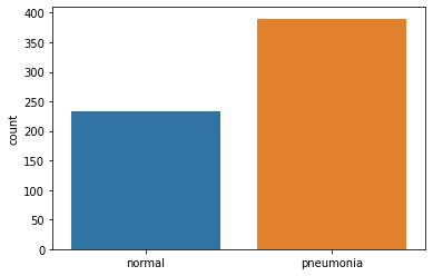
The testing dataset split into normal and Pneumonia images
We transform all these images by resizing, rotating, cropping and normalizing pixel values. Here’s the code-
But why do we even resize, crop and rotate our images? We do this to prevent ‘overfitting’. Simply put, if we train our model on the same dataset too many times, our model will begin to memorize the data given to it. It will be extremely adept at predicting labels for our training set. However, it’ll be largely ineffective at predicting the correct label for our testing dataset – our model has gotten used to the same dataset. Cropping, resizing and rotating our images randomly make them unidentical to the previous dataset, thus reducing the likelihood of overfitting.
Now you might ask, what does normalizing mean?
All images are composed of pixels. A pixel has three RGB (red, green and blue) colour channels each with a certain intensity (ranging from 0-255). These three channels come together to give the pixel a certain colour.
In order to make computation more efficient and avoid extreme pixel values from disrupting image analysis, we normalize by fitting all pixel values in the range of 0 to 1. The mean and standard deviation values given in the above code are default for all grayscale images.
Let’s look at some images now. I’ve defined a function print_img that can display these images (keep in mind that cv2 can’t display images very easily in Colab).
The first image in the training dataset. It is normal
This is the 3000th image of the training dataset. The X-ray here clearly shows Pneumonia
One can clearly see the difference between the two X-rays. The first image (index=0) has a relatively clean and dark chest with ribs one to six (anteriorly) visible. However, the 3000th image (index=3001) is filled with fluid, indicated by white colour occupying most of the left lung on the X-ray.
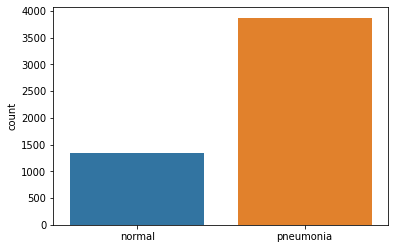
We’re done with data transformation but we aren’t quite ready yet to use this data. Our training set has 3875 images of pneumonia and just 1341 normal images. If we decided to use this as our training set our model would become biased in favour of pneumonia. We have to make out training set a bit more ‘fairer’.
If you looked at the code carefully you might have noticed that we created a train_set2, which is essentially the training set with slight modifications. The trick is to take just the normal images in train_set2 and add them in our main training set. This is the code I used to do that-
You can use train_test_split from the sklearn library to split train_set2
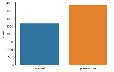
This is a graph displaying our new training set. As you can see, the number of normal images has doubled.
Another issue is that our validation set is far too small. I’ll elaborate on this set’s usefulness later, but briefly, the validation set is used to determine how well our model is performing while we are training it. It helps us fine tune our model and reach optimal prediction capacity. With just sixteen images, we aren’t going to get much benefit using a validation set – we have to increase it’s size.
Our training set right now has 6557 images. Let’s use part of this set as our validation set-
Now we have 5245 training images and 1312 validation set images. Large enough!
Finally, when dealing with large amounts of data it is always a good idea to supply images to the model in batches- we can’t give our model 5245 images to train all at once. We pass batches of images one by one to our model. Batch sizes vary, but it’s recommended to use a batch size which is a power of two.
We use a DataLoader to load batches of data to our model. DeviceDataLoader is used to transfer our dataset to the GPU (I will elaborate on this later)
Let’s take the example of a hypothetical grayscale 2D image. This image has 25 pixels (5 x 5) and each pixel has some intensity. We also have a 3 x 3 kernel with certain weights that ‘slides’ over this 2D image. It fits into each 3 x 3 section of our 2D image, multiplies each pixel of the image with it’s own corresponding value and adds all 9 values up to form one pixel.
Okay, so how does this help with our predictions? Let’s imagine this 2D image which displays a chest X-ray. The model will pass a kernel over the image and produce an output feature map. Initially, our model had to deal with 25 parameters (in form of 25 pixel intensities). By passing the kernel over this image, this model now has to consider 9 parameters instead of 25. this new feature map of 9 pixels is a weighted sum of the original image.
Let’s assume we had 10 different 2D images all with pneumonia. After looking at each image the model will be able to identify commonalities and particular features that will appear in images containing Pneumonia. Perhaps it’s a certain pixel which will have an intensity value above 0.8 if the image had pneumonia. These relationships and identifying features will be determined by our model itself (this is the beauty of ML/supervised learning – we don’t define any rules, the model simply learns itself!).
Another point to mention is that the initial weights in a kernel are randomised. The best thing about our approach (using transfer learning) is that we only need to change the final layer of our model (I will go through this in greater detail when we start looking at ResNet50). Since our model is pretrained on millions of images already, its kernels have weights that are far more suited to our X-ray images than if it was randomized.
When we introduce our testing set to our model, the model will look for these commonalities and particular features and will make a prediction!
The second step – Defining our functions
In order to train our model we need to create a few custom made functions. The first set of functions we shall define are an accuracy function, a training function, a validation function and a function that obtains the mean of our training and validation accuracy/loss.
Our accuracy function (given above) works in a very simple manner. It calculates the number of predictions that match the label (the true classification of the image) and then divides the sum by the total number of images passed to the model.
Let’s dissect our first function –
The training_step function applies our model to the images and creates an output (once again, visualise a hypothetical 5 x 5 2D image and try to figure out how the model proceeds). Self is simply a default object we have to include in our functions (refer to this link to understand it better – http://neopythonic.blogspot.com/2008/10/why-explicit-self-has-to-stay.html). It represents our model.
Okay, so what next? After our images are passed to the model we obtain two probabilities for our two classes (normal and Pneumonia). We select the highest probability and compare it to the label of the image. For example, let’s say our model predicted that the probability of an image (with pneumonia) being pneumonia was 0.3. To calculate our loss, we take the logarithm of the picked probability. If our probability is close to 1 (high) then its log value will be a very small negative number close to 0. If the probability is low (like in our case) then the log value will be a very large negative number. Multiply the two log values with -1 and we get a very large positive value (if our probability is close to zero, that is, it is a bad prediction).
The log of probability is on the Y axis. If this value is close to 0 (as in the case of a high probability), then our loss is a small positive value. If it is close to 1 (low probability) then our loss is a very high positive value.
I have specified my criterion to be F.cross_entropy but there are other loss functions you can use (CrossEntropyLoss is a commonly used loss function).
Validation_loss_a works similarly to our training_step. I’ll demonstrate it’s importance when describing the next set of functions. Our final function validation_epoch_end simply takes the average of our training loss, validation loss and accuracy and returns it.
This is our next set of functions to consider. All evaluate does is it takes a dataset (validation or testing depending on whether test =False/True). It obtains outputs by applying the model to the dataset and calculates loss. Notice that we have called model.eval() before we actually apply our model. This disables a few layers in our ResNet50 model and also turns off gradient calculation (explained in greater detail below).
get_lr is a simple function that obtains the learning rate from our optimizer’s parameters and returns it. Once again, I’ll explain the concept of learning rate (lr) below.
Now to the last bit. fit_one_cycle is the final, most powerful function that involves and uses all other functions we have defined earlier. It takes in eight arguments – number of epochs, maximum learning rate, model, training dataset (train_dl), validation dataset (val_dl), weight decay, gradient clip and the optimizer. Let’s go through fit_one_cycle line by line.
First of all, we’ve defined an optimizer, which is an algorithm by which we can reduce our loss to a minimum point. Our opt_func uses Stochastic Gradient Descent (SGD) as the optimizer.
Essentially, everything over here revolves around obtaining a gradient of our loss function. If you’ve read the code carefully you might have noticed loss.backward(). This function calculates the derivative of our loss function (dloss/dx) and then creates a gradient of this loss derivative. Our requirement is to achieve a minimum loss – we need to find the lowest point of the gradient.
An optimizer will iteratively tweak it’s parameters to reduce a function to its minimum. Gradient descent will move in the direction opposite to the steepest ascent by calculating the slope (which is dloss/dx) at every point (hence iteratively). Stochastic gradient descent is a more efficient and computationally friendly version of gradient descent.
What about learning rate? The size of steps taken by the optimizer to reach this minima is given by our learning rate. Too high a learning rate and we risk never reaching the minima.
There is a way we can prevent our lr from spiralling out of control and getting too high. We can use a one cycle learning rate scheduler to specify a maximum lr. During one whole training cycle, our lr will gradually increase, reach the max lr specified by us and then begin decreasing. You’ll also come across other schedulers (ReduceLRonplateau is a popular one) and you can use these in place of OneCycleLR and look at the results.
Weight decay is another variable I’ve introduced into the optimizer. Essentially, we don’t want our model to get too complex because that can lead to overfitting. We used data augmentation to prevent our model from overfitting on a data level. We introduce weight decay to prevent our model from overfitting on a model level.
The best way to ‘penalize’ complexity would be to add our weights to the loss function, but that isn’t very practical since our weights contain both positive and negative values. We could add the square of our weights to our loss function, but that would make our loss huge. We thus multiply our squares with a fixed weight decay to reduce their size. We reduce the value of these squares by a fixed amount (usually 0.1).
Even though I’ve displayed SGD as my optimizer over here, I will eventually change it to ‘Adam’ , another very popular optimizer. To understand more about that optimizer, take a look at this link- https://medium.com/mlearning-ai/optimizers-in-deep-learning-7bf81fed78a0. I got the above images from the same site.
Moving on, we use a for function to create a loop where a training phase and a validation phase is executed for each epoch (or cycle). Just like in model.eval(), we call model.train() to activate certain layers of our ResNet50 network.
We then create a second loop inside the first loop. Our training dataset is split into batches (one batch containing 64 images). We wrap train_dl in tqdm, which is a neat function that displays a progress bar for each epoch. For each image in a batch, we calculate the loss, obtain a gradient (loss.backward()), update our optimizer’s parameters by calling optimizer.step() and set our gradients to zero for the next batch.
You might have noticed a grad_clip function in the mix as well. Simply put, training gradients can be unstable depending on the learning rate and type of loss function. Erratic and large changes to our parameters (weights) can lead to a numerical outflow known as ‘exploding gradients’. To prevent gradients from assuming very large values or exploding out of our preferred range, we introduce an upper limit above which a gradient will be clipped. Check out this link- https://machinelearningmastery.com/how-to-avoid-exploding-gradients-in-neural-networks-with-gradient-clipping/ if you’d like to learn more about this concept.
To end our training phase, we call sheduler.step() to update our learning rate.
Our validation phase is very simple. We simply use the evaluate function to apply our trained model to our validation set and obtain our validation accuracy and loss. These results help us understand how our model is performing against new data during the training period.
The third step – Making our model
I’m using transfer learning in this project, which means that I don’t have to actually create my model by writing code. Nevertheless, it’s always useful to know about the various layers in a Convolutional Neural Network (CNN).
ResNet50 is a very commonly used model for image detection. It’s trained on the ImageNet dataset, which has over a million training images and around fifty thousand validation images. It has fifty layers (hence ResNet50) and it’s architecture looks something like this-
We start with our first convolutional layer containing 64 kernels of size 7 x 7 with a stride of 2 (think of ‘stride’ as the size of our footsteps – it determines the gap a kernel leaves when moving horizontally and vertically). We add a padding of 3 (we ‘pad’ the input image by adding extra pixels with a value of 0 to its length and height). Our input (from the ImageNet dataset) is an image of size 224 x 224, 3 colour channels (remember, ResNet50 is trained on coloured images).
Our output is normalized and is passed through a Rectified linear unit activation function (ReLU) to introduce non-linearity into our model. ReLU replaces all negative values in our tensor with 0, thus introducing a non-linear relationship between our outputs and inputs.
All our negative values are replaced by 0
Our first convolutional layer, our batch normalization layer and our ReLU function make up our first block. Our second layer is a simple MaxPool layer which has a kernel of size 3 x 3 and a stride of 2. Maximum pooling layers will consider the area a kernel occupies, take the maximum value in that kernel and create a new feature map. This reduces the size of our image – indeed, our new output feature map is of size 112 x 112 with 64 channels.
Our next convolutional block has nine layers. The first layer has 64 kernels of size 1 x 1, the second layer has 64 kernels of size 3 x 3 and the third layer has 256 kernels of size 1 x 1. A batch normalization layer and a ReLU function follows every layer. We pass our output through a batch normalization layer.
‘ResNet’ means residual network. The idea is that we add our input back to our output and make our model learn about the difference between our output and input. If we were using a traditional neural network, our model would try to learn H(x), that is, the output. However, if we were to denote the difference between output and input (x) as R(x) –
How does this link back to our convolutional block? After we’ve obtained a feature map from our inputs, we add our inputs back to this output feature map (we need to pass our input through one layer with 256 kernels of size 1 x 1 first to bring it to the same size as our output). The forms a ‘skip connection’ that skips over our three layers to reach our output.
The three layers in this block are repeated three times, giving us a total of nine layers in this convolutional block. Our new feature map has a size of 56 x 56 and 256 channels
Our third convolutional block has 12 layers. Our first layer has 128 kernels of size 1 x 1, our second layer has 128 kernels of size 3 x 3 and our last layer has 512 kernels of size 1 x 1. Again, we add our input back to our output to obtain a residual block. These three layers are repeated four times. Our new feature map has a size of 28 x 28 and 512 channels.
The fourth convolutional block (another residual block) has 18 layers. The first layer has 256 kernels of size 1 x 1, the second layer has 256 kernels of size 3 x 3 and our third layer has 1024 kernels of size 1 x 1. This is repeated six times and our resulting feature map is of size 14 x 14 and 1024 channels.
Our last convolutional block (you guessed it, another residual block) has 9 layers. It’s first layer has 512 kernels of size 1 x 1, the second layer has 512 kernels of size 3 x 3 and the third layer has 2048 kernels of size 1 x 1. This is repeated thrice and our resulting feature map has a size of 7 x 7 and 2048 channels.
We have one average pooling layer (which works similar to the max pooling layer, only that the kernel will take the average value of all elements within it) which reduces the size of our feature map from 7 x 7 to 1 x 1. We also flatten our feature map to get a output of size 1 x 2048.
Our final (and in practice the most significant layer) is a fully connected layer attached to a softmax function. This layer will reduce the number of channels to the number of output features (labels) we require. The original ResNet50 model has a fully connected layer with a thousand nodes, but we only want a result which has two values (probabilities for label pneumonia (1) or label normal (0)). To achieve just two nodes, we replace our last layer with our own custom built fully connected layer –
num_classes is equal to two
I’ve mentioned a ‘softmax’ function as well. This is a very crucial function that converts our results into a probability. We need our results to lie between 0 to 1 and add up to one. Softmax replaces every value (y) in output by e^y and then divides this by the sum of values to ensure that this adds up to one.
Okay, so we’ve finally made our model. All layers except the last fully connected one are untrainable – we cannot change the parameters (weights and biases) of those layers. Our training mainly affects the last layer. My explanation might have been confusing, so if you’d like some more clarity check out this YouTube video I found to be very helpful- https://www.youtube.com/watch?v=mGMpHyiN5lk
The fourth step – training our model
This is the fun part – we get to see our model perform on training and validation data and utilise all that we’ve coded.
We begin by evaluating our model’s performance against the validation dataset-
Since we haven’t actually trained our model, the validation accuracy is quite bad. Statistically, if we just randomly guessed we would be able to reach an accuracy of 50%. Let’s train our model and look at the improvements.
Before we begin, have a look at our fit_one_cycle function. It requires the number of epochs, a max learning rate, a gradient clip value, a weight decay value and an optimizer.
Wrapping our data with tqdm gives us some other pieces of information and lets us track our progress in each epoch-
That’s how our training looks. We can see that by epoch 14 (remember, our first epoch is designated epoch [0], so I am referencing number [13]) our training loss, validation accuracy and validation loss has stabilised.
Refer back to the fit_one_cycle function. I had created empty lists for training loss, validation accuracy and validation loss so that each value would get stored into their respective lists. These values can be used to plot line graphs illustrating the performance of our model over time.
The fifth step – testing our model
Let’s look at how our trained model performs against our test set-
Not bad! We’ve obtained an accuracy of 93.4% We could potentially improve this by altering the number of epochs, batch size, max lr, weight decay, gradient clip or optimizer.
Let’s have a look at the confusion matrix for this test set –
I’ve always found a confusion matrix to be the best way to visualize a model’s performance (in real terms). Here’s the code if you’d like to make your own confusion matrix-
Let’s look at our model’s predictions for various images-
Our model predicts the first image of our testing dataset correctly!
Our model predicts the 451st image of our testing dataset correctly!
Let’s look at an image our model couldn’t predict correctly-
This image (17th in our testing set) is fairly distorted and isn’t very clear. It’s understandable that our model couldn’t predict the right label.
Let’s also have a look at line charts displaying our model’s performance-
This graph above shows the variation of training loss over epochs. We can see a general downward trend- our model gets better at predicting images and thus the total loss decreases. By our 14th epoch the loss has stabilised.
This graph above displays our validation accuracy over epochs. Our validation accuracy was a bit erratic in the beginning but stabilised around epoch 14. It does, however, have an overall trend upwards.
This graph displays our validation loss. The general trend is downward, but it is fairly erratic in the beginning.
GPUs vs CPUs
GPUs make your life much easier – when training on CPUs each epoch took around six minutes to train. Twenty epochs would take at least two hours to complete. With a GPU, twenty epochs are completed in just over six minutes.
A great thing about Colab is that it gives you access to Google’s own GPUs. However, this access is quite limited and getting access to GPUs usually depends on luck. If you have a computer with a GPU, you can use that (if you want to use Colab, change your runtime type to GPU). You’ll also need to write some code to utilize your GPU-
We’ve defined a to_device function that will move data or models to our GPU. This is very important- if your data is in the GPU but your model is still in the CPU you will get an error. For example, we need to move our model to our GPU by simply writing –
My reflections on this project
There were many things I learned while doing this project. It gave me an opportunity to think about what I want to achieve from coding and think about how ML could change medicine.
First of all, I learned that attention to detail is particularly important – unfortunately, I learned this the hard way. For nearly two weeks my code returned the same testing accuracy of 62.5%. I tried and tried to solve this but couldn’t figure out why my training and validation set had 97% accuracy but testing remained that low. I realised my mistake when I looked at the mean and std values I had used to transform my testing dataset. Turns out I had used a wildly incorrect set of std values for the test data, resulting in the complete corruption of all images in that set. If I had paid attention to detail and checked my code line by line, I would’ve spotted this discrepancy ages ago!
Another thing I learned was about getting help. I discovered the go-to forums and platforms where you can ask your questions. Stackoverflow, Python discord and Jovian helped me whenever I couldn’t proceed. Talking to people who are familiar with code/Python also helps.
Finally, I now appreciate the importance of understanding concepts and underlying algorithms. Just knowing how to write code isn’t enough – one must have a keen understanding of how various algorithms and functions work. You must be able to visualise the whole process. Reading articles related to these concepts is a must.
ML in medicine is a new area for me, and even though my knowledge is limited, I have done some reading in the subject and would like to now give my perspective on how ML might have an impact on healthcare.
My understanding is that ML will become a part of the consultation of the future. It won’t replace healthcare professionals (or at least I hope it doesn’t!) but it will assist in the decision making process. For example, a program might make a parallel diagnosis and alert the doctor if their diagnosis and the program’s diagnosis doesn’t match. We might also see ML assisted healthcare being deployed in areas of the world that don’t have access to proper medical services. The applications are endless.
Of course, making diagnosis is a very complex affair. Doctors consider many aspects of a patient’s history to reach a decision. They tend to notice other things (a change in the patient’s walking style, demeanor, etc) that a program simply can’t do. However, technology moves at a blisteringly rapid pace. We may not have the ability to definitively diagnose patients using ML now, but that milestone will almost certainly be reached in the not-so-distant future.
This also brings me to another point I want to mention – doctors and healthcare professionals alike must also change and adapt to the presence of ML in the healthcare environment. They must also make an active effort to understand the software and take part in the design stages of these programs. It is imperative that doctors shed the idea that all they are meant to do is diagnose and treat. I do not mean to say that doctors must start learning how to code. However, they must be able to grasp the basic ideas and concepts that power a program and must get involved in the software production stage. As opposed to simply being advisors to a team of software engineers, doctors must be the people who define what a program should achieve and demand features and improvements (this approach would ensure that doctors remain in control – ensuring that the patients best interests are always of paramount importance).
Moving on, drug discovery is another area of healthcare that might see paradigm changes through ML. Bioinformatics and Cheminformatics are perhaps not as ‘chic’ as autonomous surgical robots or disease prediction programs, but their potential can in no way be understated. Today it takes researchers many years to find the correct mix of molecules that could make an effective (but not toxic) drug. Bioinformatics and Cheminformatics might actually make this process quicker and cheaper (I did a short course of Bioinformatics as well – I found it very interesting!).
We tend to see supervised learning as the dominant ML subcategory in healthcare. This makes sense- it’s probably better to use a data driven approach since that doesn’t require experimentation or major assumptions on the model’s part. Reinforcement learning (RL) hasn’t made many inroads in healthcare in part due to this- it would be very irresponsible to use Temporal Difference learning to bootstrap and make assumptions regarding future results of a certain treatment.
However, I do think that we’ll slowly see RL making inroads in medicine as well. I envision it being used primarily in drug discovery. We could define a goal of creating a compound with low toxicity and high effectiveness. Any step taken (for example, the addition of a particular molecule) that contributes to the compound’s efficacy would result in the model getting a reward. It will thus attempt to find those combinations that maximize its rewards (if you are really curious about RL have a look at this course by UCL Professor David Silver – link).
What next for me?
I’m really happy with this project, but I do understand that in the spectrum of complexity, it is on the less difficult side. My plan for the future is to learn Python and do projects in tandem, while gradually increasing the complexity of each project. I’m currently doing a course on Liver segmentation using Monai, which is a library specifically for medical imaging. I’ve also created a playlist of all useful courses and videos I seen on Python (I would suggest this for everyone who’s staring with coding) since it allows me to keep track of what I’ve done and what I plan to do next.
This has been a very long blogpost, I think it’s a good idea to end it here. I hope it’s been a good read and has motivated you to learn Python and do a project of your own!
Most aircraft today fly at a height of 30000 feet above ground. Sitting inside the jet, we experience surface-like conditions, along with the usual ample supply of air. However, there are some people who reach these heights on foot, braving the cold, lack of oxygen and the many crevasses and tumbling rocks that could harm them. People look to mountaineering as an exciting hobby – something that will allow them to discover more about themselves as well as push their bodies to the limit. Very few peaks are as coveted as the grand Everest, known in Nepal as ‘Sagarmatha’.
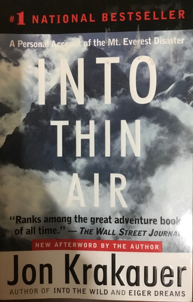
My copy of ‘Into Thin Air’
However, not all those conquering Everest are seasoned mountaineers. The past three decades have seen the rapid commercialization of the mountain. Many experts considered and still consider this to be quite dangerous. In the May of 1996, their words came true, when 12 people died attempting to scale the summit. ‘Into Thin Air’ is a story of that disaster written by journalist Jon Krakauer, one of the members of an ill fated Everest expedition group.
A long waiting line on Everest- a consequence of the commercialization of the mountain
The book is a gripping thriller, with each page revealing some mistake or the other that contributes to the deaths of many climbers. I was quite interested in the medical aspects of the issues faced by climbers- HACE (High Altitude Cerebral Edema), HAPE (High Altitude Pulmonary Edema) and frostbite seem to be some common issues doctors at the Everest Base camp have to manage. Since these conditions were very new to me, I decided to explore them and their underlying reasons more closely.
Most climbers who aren’t acclimatized (another word for adapting to the lower oxygen availability) will face some type of altitude sickness. At higher levels, the concentration of oxygen remains the same as sea level concentration – roughly 21%. The problem is that oxygen molecules in air are in short supply. With less oxygen entering the body, organs are deprived of this life giving element. This leads to a variety of problems- nausea, vomiting, light headedness and tiredness are usually seen. This lack of oxygen also explains why certain illogical decisions were made by the climbers at Everest – thin air severely impairs one’s ability to think. It essentially clouds the mind, thus making seemingly obvious decisions terribly hard to make up there.
Sherpas, on the other hand, are well suited to make trips up Everest whilst carrying back breaking loads. Their bodies are used to high altitudes, thus they are ever acclimatized to their surroundings.
HAPE and HACE occur when blood vessels in the lungs and the brain (respectively) begin constricting. This is a natural response to the cold- vessels constrict to reduce blood flow and conserve heat. However, the constriction of blood vessels increases the blood pressure, which in turn results in the leaking of fluids into the lungs (and in HACE, into the brain). Symptoms of HAPE include a persistent cough with sputum, difficulty in breathing and a blue tinge in the lips or skin. Those of HACE include confusion, headaches and fever. Dale Kruse, who is mentioned in Into Thin Air as a climber who suffered from HACE, described his condition as being extremely drunk.
Into Thin Air was a wonderful read. From miraculous survivals to teary deaths, it is certainly a book that you will get riveted to. I especially enjoyed reading about the daring helicopter landing done by the Nepali air force- the fact that helicopters could fly in that thin air amazed me!
Written by bestselling author Adam Kay, ‘Twas the nightshift before Christmas’ is a hilarious, horrifying and often heartbreaking book that will surely bring a smile to your face. Kay delves back into his junior doctor diaries once again, this time focusing on the many Christmases he spent in the hospital, away from friends and family.
The book is filled with many rib-tickling experiences that Kay has had. One such amusing experience that he has written about is when his tie (which had a sound piece) started screaming out a Christmas Carol during a tense session with an elderly patient’s family. His frantic efforts to switch it off only made the song repeat, but he finally succeeded in getting rid of the sound.
Apart from the jokes, the book also makes us appreciate the millions of healthcare workers who give up their enjoyment and holidays to tend to the sick and injured. Much like soldiers, they too have to be ever vigilant and ready to serve, sacrificing many comforts. The book also displays the passion Kay had towards his profession- even though he used to curse his luck and rota schedule for making him work on Christmas, we learn that he misses the nonstop shifts and ungodly hours he had to work in.
All in all, this book is a wonderful read. I’d certainly recommend this (and his first book, ‘This is Going to Hurt’) to all aspiring clinicians- It acts as a fitting tribute to all healthcare professionals around the world who sacrifice their time to ensure that every person is safe.
Anatomy in general is quite interesting, and a fish dissection is an activity that allows one to explore and learn. It also helps one develop a better understanding of the human anatomy as a whole.
While fish anatomy isn’t human anatomy, it’s not extremely difficult to find areas of similarity between the two. For instance, the intestine of a fish is quite long and convoluted, just like a human intestine. I’ve done a couple of dissections myself, and have found that my understanding of anatomy did get better. If you’re looking to do your own dissection, look no further! I’ve listed the steps below. Have fun reading!
Just a reference image
STEP 1
Find your fish. I prefer using the Catfish, since it’s quite easy to cut open. Another alternative is Milkfish, though I haven’t used one myself.
The catfish
STEP 2
Find your instruments. You will need a scalpel, a needle, a scissor and a tweezer. I recommend wearing gloves and a mask. You might want to get some air freshener as well (it gets really smelly, so if you can, do it outdoors).
My kit
STEP 3
Using your scalpel, make a light cut on the underbelly of the fish starting from the anterior end. Extend it all the way back towards the posterior end. If your cut isn’t deep enough, go back and do it again. If you widen the gap, you’ll be able to see the internal organs. The first thing you should encounter is the stomach.
The first cut. I didn’t extend the cut up to the anus (the tiny hole) but I should’ve done so
STEP 4
After encountering the stomach, you can go ahead and remove it. If you carefully analyse its contents, you might find some digested food (maybe smaller fish). Go ahead and remove the intestines. I did this using the tweezers. Try being gentle, otherwise you may end up breaking it.
Out with the stomach
STEP 5
Keep exploring. Widen the gap you’ve made and look into the anterior cavity. You can find a very dark red organ- the fish liver.
The dark blob one can see is the fish liver
By this time the cavity should be quite empty. Look inside- there will be a large white structure (you can’t miss it!). It’s pretty rubbery. This is the swim bladder, used by the fish to maintain a specific depth. You’ll have to use your hands to remove this, since it’s attached to the dorsal wall. Now extend you original incision towards the anterior end till you reach the point shown below.
If you’re lucky, you’ll also find the heart (it can be a bit hard to find. I didn’t get it in this dissection, but I did find the heart of a different bony fish I’ve forgotten the name of).
The two chambered heart of a fish
A fish heart is quite different as compared to a human heart- while the latter has four chambers (Right Atrium, Right Ventricle, Left Atrium and Left Ventricle) the fish heart only has two chambers (an upper atrium and lower ventricle). Another interesting fact is that while the human heart has a double circulation system (blood flows in two circuits – from the heart to the lungs and back and from the heart to the body and back), a fish has a single circulation system. In a nutshell, blood follows this pathway – body to heart to gills to body. Blood does not return to the heart a second time.
STEP 6
Onto the eyes and gills. The gills can be a little difficult to remove since they have a flap called Operculum covering them. You can use your hands to access the gills.
An interesting fact about these gills is that they use Counter Current exchange – a mechanism which involves exchange of liquids between two bodies flowing in opposite directions to each other. The capillaries in the gills flows in a direction opposite to that of water, thus creating this very mechanism. Nephrons in the human kidney use a similar mechanism to concentrate urine.
The eye is actually quite interesting. Though I haven’t tried it myself, you can remove most of the slimy layer and obtain the near circular lens of a fish. If you hold it up to a light, you’ll be able to see how light passes through lenses and flips the image upside down.
STEP 7
Clean up. It’s not the best part of the dissection but absolutely necessary. You might want to get rid of the smell too. It helps if you have a cat (I hear they like fish).
Overall, I had a lot of fun doing this dissection. It’s something entertaining as well as educational that one can do in the lockdown. I hope you enjoyed reading this blog post!
Neurosurgery is a specialty that has always intrigued me- the human brain is a complex, unique and fascinating organ, and those who treat it require years and years of training, along with the ability to withstand significant mental and physical stress. Few books cover a neurosurgeon’s life as well as ‘Brain Surgeon’ written by Dr. Keith Black.
One can really understand the passion and love Dr. Black feels for his profession. He often compares the brain to tiger country, where each step taken requires vigilance and alertness. To him, the brain isn’t just any other organ- it is the most unique thing about our body. It’s ability to rationalize, think, remember and communicate is the reason for humankind’s success as a species.
My copy of ’brain surgeon’
Another aspect of the book that I loved was that he has made this work his tribute to each patient he has ever treated. As a neurosurgeon specializing in treating tumors, most of his patients cannot be cured completely. Often, surgery only extends the life of a patient by a few months. The reader comes to the realization that these patients are suffering from diseases that are usually fatal. This is why learning about patients like William Tao, who remained jolly and resilient in the face of adversity, is quite heartwarming.
The last chapter, however, is the most significant part of the book. Dr. Black tells us the fate of each patient he described. As it turns out, most, while having been given a temporary lease of life, are heading towards inevitable demise. William Tao, the optimistic and happy patient I mentioned above, dies of his tumor. Dr. Black, rather than listing out his many achievements, lists out those he couldn’t save, impressing the fact that while medicine has innovated and evolved to a great level, there are still situations where our best efforts often do not succeed.
Allow me to take you on a journey to a typical surgical theatre of the 1850s. While making your way to the theatre, you see the windows of the hospital being opened and hear the words ’Miasma.’ As you enter the theatre, you hear the cries of a writhing man on a dirty operating table. The man has been restrained by three people, while a surgeon wearing a stained coat saws through his leg with a saw (which, mind you, has dried blood on it’s blade). On the side is kept a box of sawdust for the leg, sand to soak up the blood and a stove that heats hot irons which help in stopping bleeding.
Baron Lister, 1902
While akin to a scene from a horror movie, this is very much like the operating theatres of the 1850s. No medical professional believed that hygiene was an important part of their job. Surgeons used to believe that the amount of stains on their coat was an indicator of their experience. Most of all, the instruments they used were never washed, being used again and again for procedures. However, there was one clever person who, inspired by the work of the French Louis Pasteur, was going to change how surgery took place for the better.
Often hailed as the father of modern surgery, Joseph Lister was born on April 5th, 1827 to a prosperous Quaker home. His father had been a pioneer in the development of achromatic lens for compound microscopes.
Lister didn’t immediately obtain his degree in medicine, having completed a Bachelor of Arts degree in Botany from the University College London. He then went on to study medicine and graduated from the Royal College of Surgeons.
During Lister’s time, people used to believe that infections were caused due to ’miasma, ’ or bad air. Hospitals were occasionally ’aired out’ to remove this miasma from the wards (if you were confused about the part in which windows were opened in the first paragraph, I hope this clears stuff up). There were virtually no facilities to wash hands.
Lister, now a professor at the University of Glasgow, read a paper published by the French chemist Louis Pasteur, which showed that food spoilage could occur under anaerobic conditions (anaerobic essentially means without oxygen) if micro-organisms were present. Pasteur recommended three methods to remove bacteria – filtration, exposure to heat (what is now widely known as Pasteurization) and exposure to chemicals. After confirming Pasteur’s conclusion himself, Lister decided to use the third method (treatment of chemicals) since the latter two couldn’t be used on a patient.
After hearing about a certain chemical known as Carbolic acid, Lister decided to test it’s ability to remove microbes. He began spraying the acid on instruments, dressings and incisions. On applying it to wounds, he found that the incidence of Gangrene (death of tissue due to bacteria infection) was greatly reduced. The final confirmation regarding Carbonic acid’s effectiveness came when he applied it in a seven year old child named James Greenless, whose leg had been crushed under a hay cart, breaking his bones. Six weeks later, the child was walking without any support, bones healed, with no infection or pus near the now healed wound. With this overwhelming success, Lister published his findings in the Lancet, the leading medical journal of the 1800s. His paper recommended surgeons to wash their hands in a 5% Carbolic acid solution, along with spraying of this solution on surgical instruments.
Lister’s Catholic steam spray apparatus
Now Lister was quite fortunate in some aspects. His paper, while criticized initially, made him famous around the medical field. His fame as the person to make surgery safer granted him the title ’father of modern surgery’. He was appointed surgeon to Queen Victoria and was raised to the peergae of Baron Lister. He retained his position as surgeon to the monarch during King Edward VIIs reign. The King, having developed appendicitis two days before his coronation, was treated with the latest antiseptic methods on the recommendation of Lister. Unlike Ignaz Semmelweis, a physician who tried to implement antiseptic treatment before Lister, he did not end up in squander.
Lister’s ’On the antiseptic principle in the practice of surgery’, The Lancet, 1867
Of course, while Lister’s contribution to surgery was of paramount importance, it was just the start. As the years flew by, Surgeons implemented a sterilized surgical theatre, strict handwashing, sterilized surgical instruments and the usage of sterilized surgical gowns, masks and gloves, bypassing the need for any disinfectant. The innovation of anesthesia by American dentist William Thomas Green Morton paved the way to a greater number of surgical procedures that could be performed. As the healthcare sector innovates rapidly, the contributions of Lister and other pioneering surgeons must never be forgotten, as it is their work that has given us safe healthcare today.
By this time, I’m sure most of us have already seen the coronavirus structure. It’s sort of like a ball, but far less fun to play with. While we’ve seen the virus in pictures, scientists at Massachusetts Institute of Technology have used this structure to produce music!
The music that you hear represents the various aspects of the virus shape. The spikes that one can see are actually made up of Amino acids, the building blocks of proteins. Using a technology known as Sonification, the scientists assigned each acid to a unique note in a musical scale, effectively composing a new and rather strange sounding musical score played by a Japanese Koto instrument.
However, the notes aren’t actually made by the widely known ball with spikes coronavirus structure. In real life, Amino acids usually curl up in helixes or into sheets. These features are captured by researchers by altering the duration and volumes of the notes. Vibrations on the molecular level caused due to heat are also allowed their own sounds.
The curled Amino acid structure. Source- Sciencemag.org
Now this music wasn’t just made to get an entertaining take to an image that causes terror. This new format could help scientists find sites on the protein (an Amino acid, as stated above, is the building block of proteins) that antibodies and drugs can bind to. This is done by searching for very specific musical sequences that can correspond to the sites on our musical score. This, researchers say, is a faster method to study proteins as compared to more conventional methods such as molecular modelling.
While efforts to understand the structure of the coronavirus on a molecular scale are ongoing, many pharmaceutical companies and universities are beginning to start trials of new drugs. Many older drugs are also being touted as a possible cure, most popular of which is Remdesivir, a drug originally intended to cure Ebola, but is now showing favourable results in monkeys. Another drug widely believed to have a shot at curing the virus is Hydroxychloroquine, a Malaria drug.
While scientists worldwide are vigorously researching the possible cures and doctors, nurses and other healthcare professionals are spending days and nights in hospitals tending to those infected, the best way to prevent infection is to stay at home, wear a mask when outside and regularly wash their hands. Soap has been heralded as the most effective weapon against coronavirus, being able to dissolve the virus’ fat membrane that encloses its genetic material.
Have you ever wondered how the different parts of a flower look like? We’re quite accustomed to seeing the beauty of a flower with all its petals, but a flower is an amazing object even on the microscopic level.
Now, you might want to explore a flower in more detail yourself, specially if you’re #stayinghome and are getting bored (if you are, get a flower from your garden, don’t step outside!). You’ve come to the right place! I’ve given the steps to a flower dissection below. I did this myself and got some really impressive results!
Step 1) Obtain your flower and instruments. Now while this might seem as a easy step, one must realize that you can’t use any flower. You’ll need one which has all its organs intact and visible. It should ideally be a bisexual flower, which has both stamens (the male organ) and carpels (the female organ). I used a Hibiscus flower. As for the instruments, you’ll need a needle, tweezers and a blade (not as important, but it helps if you have one).
There’s the flower. The anthers and the four stigma are visible.
Step 2) Get familiar with your flower. Learn its various parts first. You’ve got the sepals (the small green structure at the base of the flower which protects the bud before it opens), the petals, the stamen (the stamen is composed of the anthers and the filament. In Hibiscus our filament is the long red stalk that emerges from what seems like a dark hole. The anthers contain pollen, which is the yellow stuff in the picture). The Carpel contains the stigma (the four small round balls on the top), the style (which will be revealed when you cut open the filament) the ovary (the swollen green structure at the base which you’ll find after you remove the petals) and the ovule (the eggs, contained inside the ovary).
Step 3) Begin by removing the sepals. Gently make an incision with your needle and pull the sepals carefully using your tweezers. Be very slow while doing this. After you’re done, your flower should look like this-
Notice the white structure that is revealed after removing the sepals
Step 4) Remove the petals. You’ll get a flower that looks like this-
The petals are gone!
Step 5) Here comes the serious section. Use your needle to make an incision to the bottom white part. Be very careful in doing so- don’t cut too deep. After doing this, gently increase the gap that you’ve created and use the tweezers to pry out a white tube. This is your style.
Look closely and you’ll see the white tube
Step 6) Now, use your needle to cut a gap through the filament. Start the gap from the upper end of the incision you’ve made to the white structure. Keep extending it till you reach the top of the filament, being careful not to damage any part while doing that. Use your tweezers just like in step 5 to pull out the white tube. Here’s how your flower should ideally be looking-
If you’ve done this right, congrats! You’ve just got through the toughest part.
Step 7) use your tweezers to pull the filament out of it’s base. Basically, extend your first incision to the white structure and use your tweezers while pulling it in a circular fashion. You’ll have a flower (or at least what’s left of it) that looks like this-
Here, you’ve separated the two reproductive organs! The one on the bottom is the female organ while the one on top is the male organ. The white pear like structure at the very bottom above the epicalyx is the ovary. On the bottom left you can see a rifle I’ve drawn that I can’t rub off my table.
Step 8) Almost done! Cut the white style (I didn’t want to). Use a blade and cut the ovary in half, but keep both halves attached to their base. You can use a needle too, but it won’t be as neat.
Use your tweezers and gently separate the two halves of the ovary. Have a look inside – you’ll find many white round structures. These are the ovules, or the eggs. During fertilization, the pollen from the anther travels down the stigma and fuses with the egg forming a diploid zygote, a process known as fertilization.
Now we’re done with the dissection. However, if you’ve got a microscope at home, you can brush off some pollen, remove a stigma, get hold of an ovule and analyze them under the microscope. Here are some pictures I took of the pollen, stigmas and ovaries under the microscope-
The pollen grains. Observe the structure of the pollen. It looks a bit like a ball with spikes all over, and that structure helps it stick to stigma and vectors (any element that helps in transferring pollen to the stigma. Of course, I’m not saying that pollen sticks to wind. I’m referring to vectors like birds and insects).This is a picture of the stigma! I was fortunate enough to find some pollen already stuck to it.The ovules
I immensely enjoyed doing this dissection. I learnt a great deal of things, including the structure of a flower and the fact that I have to clean my microscope lens. I’ve attached the link to the video I used to do this. Hope you’ll find it useful and had fun reading this blogpost!